Mapping Chaotic Gravitational Basins

Restricted $n$ -body basins in $n$ dimensions

Nirav Ramdhanie · September 2026 · source

Collision basins for three equal masses on an equilateral triangle: red, blue and green regions with radial filaments. — Figure 1. Restricted 4-body system — three fixed planets, collision basins coloured by which planet each asteroid hits. Settings: geodesic flag false, time-to-hit flag false.

My misconceptions

I thought that gravitational basins look like Figure 2. The three white dots are “planets” not affected by each other’s gravity, and each coloured section is their respective gravitational basin. If we place an “asteroid” anywhere within the green section (with initial velocity of 0), it will fall into the green planet… is what I thought would happen. But I took a good pondering session...

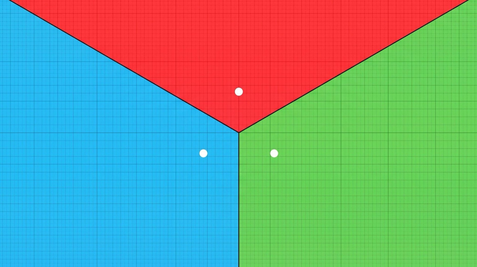
A clean three-colour Voronoi-style diagram with three white dots — the naïve picture of gravitational basins. — Figure 2. What I wrongly assumed the basins would look like — a tidy Voronoi partition.

I completely negated the fact that all planets are influencing the gravitational field which the asteroids are placed in. Meaning there is a very plausible chance where asteroids could completely miss the closest planet and orbit the system and could possibly end up colliding with any of the planets. The closest planet doesn’t necessarily guarantee the asteroid colliding with it.

So I decided to build a GPU simulation of the restricted n-body problem: a system of $n$ bodies where $n-1$ are fixed masses, and the last is a particle of negligible mass influenced by the gravitational fields of the fixed masses. I will refer to the fixed masses as planets and the negligible mass as asteroids. The asteroid moves in Euclidean $n$ -space under Newtonian inverse-square gravity until it collides with a planet of a finite radius, or until the maximum allowed time by the simulation has passed (cutoff time). I will send an asteroid for each pixel or lattice point and it will be coloured by which planet it hits, or optionally by how long that takes. This will ultimately return an image of the gravitational basins for this system.

The physical model

Since the planets do not move, they do not define a self-consistent gravitational $n$ -body spacetime, and they do not define a circular restricted three-body problem either. They are fixed “wells”. Each asteroid at position $\mathbf{x}$ feels

\mathbf{a}(\mathbf{x}) = \sum_{i} G\, m_i\, \frac{\mathbf{p}_i - \mathbf{x}}{\lVert \mathbf{p}_i - \mathbf{x}\rVert^{\,e}}, \qquad e = 3,

with default $e = 3$ (inverse square), even when the ambient dimension $n$ is greater than 3. This was a modelling choice. Gravity as in three-dimensional space, embedded in a higher-dimensional Euclidean space, not Gauss’s law in $n$ dimensions (which would fall as $1/r^{\,n-1}$ ).

All asteroids start at rest. A collision is counted through a true geometric collision with an $(n-1)$ -sphere of radius $R$ . There is a line segment created from the previous position of an asteroid to the current position of the asteroid between each time-step. If this line collides with a planet, then the first planet intersected will be counted as a collision. Motion is integrated with per-particle RK4 on the GPU; near a surface the step is CFL-limited so it cannot jump over the sphere. The initial position is coloured the same colour of the planet. If an asteroid reaches the maximum time $t_{\max}$ it colours the initial position black. This ultimately colours the image with the gravitational basins.

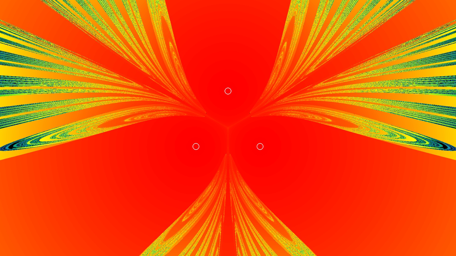
An optional map colours by collision time over $[0,\, t_{\max}]$ . I basically added this just to see how it looks, and it’s pretty cool.

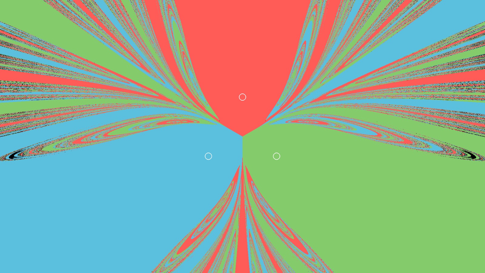
The same system coloured by time-to-hit: red interiors collide quickly, yellow-green filaments take much longer. — Figure 3. Coloured by time-to-hit (red is fast, the filamentary sea is slow). Settings: geodesic flag true, time-to-hit flag true.

An optional first-post-Newtonian geodesic flag exists since I was also curious. It is geodesic motion in a prescribed static multi-mass potential. I am not using general-relativistic three-body physics here.

Collision basins with the geodesic flag on — visibly different filament structure from Figure 1. — Figure 4. The same system with the geodesic flag on. Notice the physical difference between Figure 1 and Figure 4. Settings: geodesic flag true, time-to-hit flag false.

The VisPy desktop viewer: a 3-D cube of coloured points with a control panel for slices, planes and planets. — Figure 5. The same basins visualised in 4-D — a 3-flat through the cube of initial conditions. Settings: geodesic flag false, time-to-hit flag false, visualised in 4-D.

Why rotations don’t increase linearly

I had a problem, or really just a question. What is the most efficient way to describe a cube in $n$ -dimensional space? The reason why I needed this is because I wanted to visualise higher dimensions of gravitational basins. The cube is the 3-dimensional window that you can view. A 3-dimensional cross section. I originally thought that the set of rotations increases linearly as the dimensions increase. I soon found out that I was very wrong once again.

Translations in $\mathbb{R}^{n}$ have $n$ degrees of freedom: one per axis. Rotations don’t act the same way. The group of orientation-preserving rotations of $\mathbb{R}^{n}$ is the special orthogonal group $SO(n)$ : real $n \times n$ matrices $R$ with

R^{\mathsf{T}} R = I, \qquad \det R = +1.

The constraint $R^{\mathsf{T}} R = I$ is equivalent to the columns being an orthonormal basis. Infinitesimally, $R = I + A$ with $A$ skew-symmetric ( $A^{\mathsf{T}} = -A$ ). A skew-symmetric matrix is fixed by its strictly upper-triangular entries: one independent number for each unordered pair of axes. There are $\binom{n}{2}$ such pairs, so

\dim SO(n) = \binom{n}{2} = \frac{n(n-1)}{2}.

That is quadratic in $n$ . Each pair of coordinates spans a plane and each plane carries its own rotation angle. In 2D there is one plane and one angle. In 3D there are three planes (yaw, pitch, roll). In 4D there are already six independent rotations. 10D has forty-five of them, and so on.

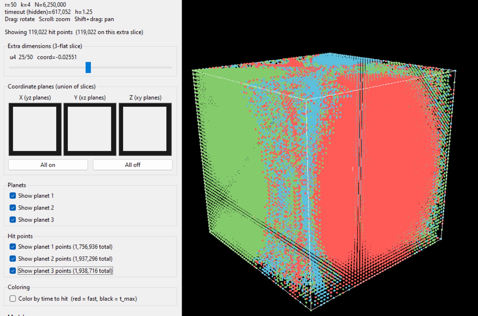
That is why a 2D image of this system is a 2-flat (an affine 2-plane) in $\mathbb{R}^{n}$ , simulated with one asteroid per pixel, after which the motion is still $n$ -dimensional. A 3D view is a 3-flat through an $n$ -dimensional cube of initial conditions. Extra axes are chosen with sliders. An $(n-1)$ -sphere of radius $R$ meets a 3-flat in a ball of apparent radius $\sqrt{R^{2} - d^{2}}$ , or not at all if the centre is farther than $R$ from that flat. It is also possible to do mixed-dimension planets: a 3D mass in 4D sits at $w = 0$ by padding.

A plain white wireframe cube on black — the 3-D viewing window. — Figure 6. The cube that took a lot of effort to build.

What the basins actually look like

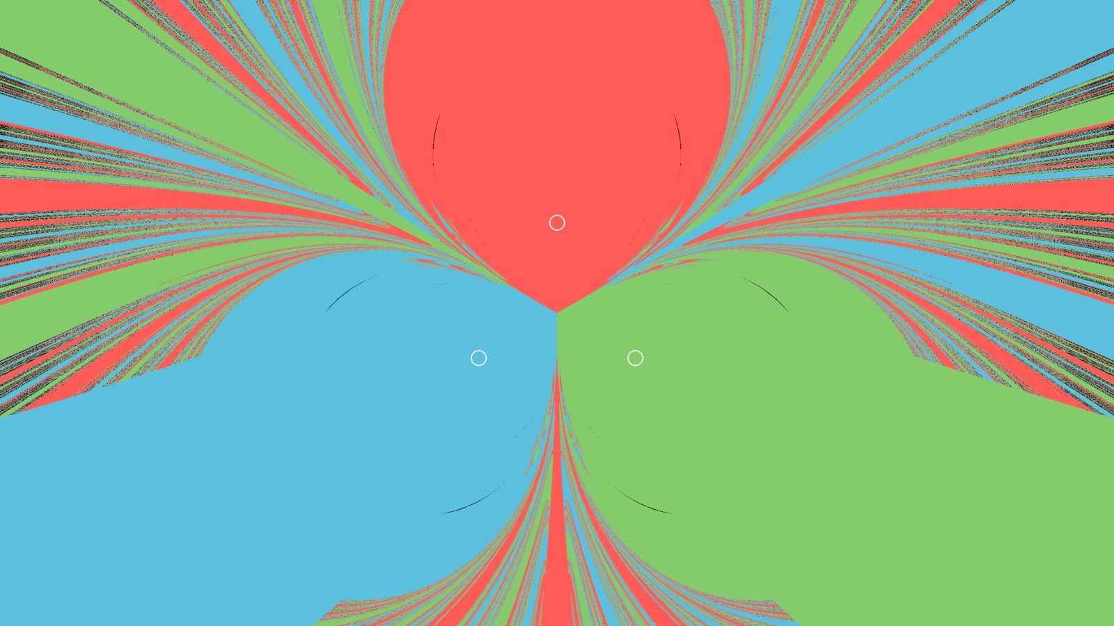
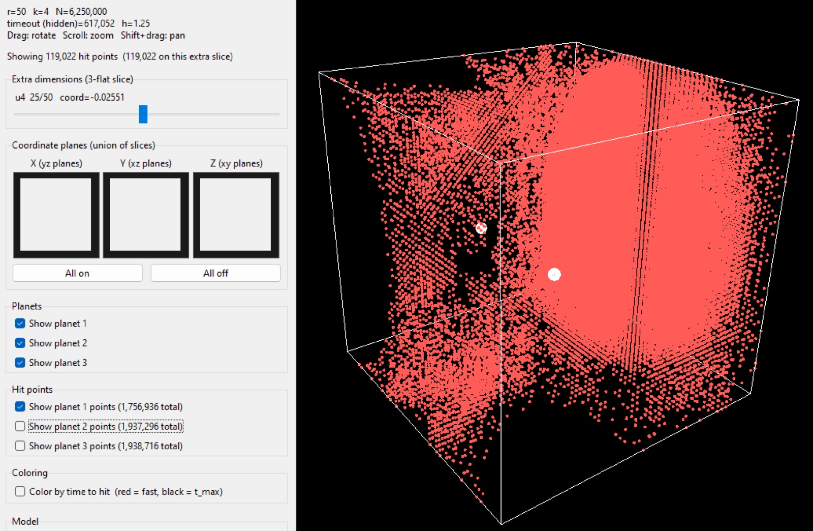
See Figures 1 and 5. I pretty much did simulations for just one system: three equal masses on the vertices of an equilateral triangle. As I figured out, the collision map is not a Voronoi diagram. If you zoom in, each planet has a compact capture region analogous to a Roche lobe. Far away the combined field is nearly that of a point mass, so a particle that starts at rest falls almost radially. Which planet the asteroid eventually hits is decided by tiny deflections as it threads the triangle. The far-field therefore looks like radial stripes. Between those two effects, the boundary is very chaotic.

That structure is a basin of attraction in configuration space (here the space of initial positions at zero velocity). The images show the hallmarks of Wada basins: the boundary of each colour appears to be a boundary of all colours. A set $W$ is a Wada boundary if every open neighbourhood of a point of $W$ intersects every basin. Then there is no “edge between only red and blue”. Any neighbourhood of the edge contains all red, blue, and green.

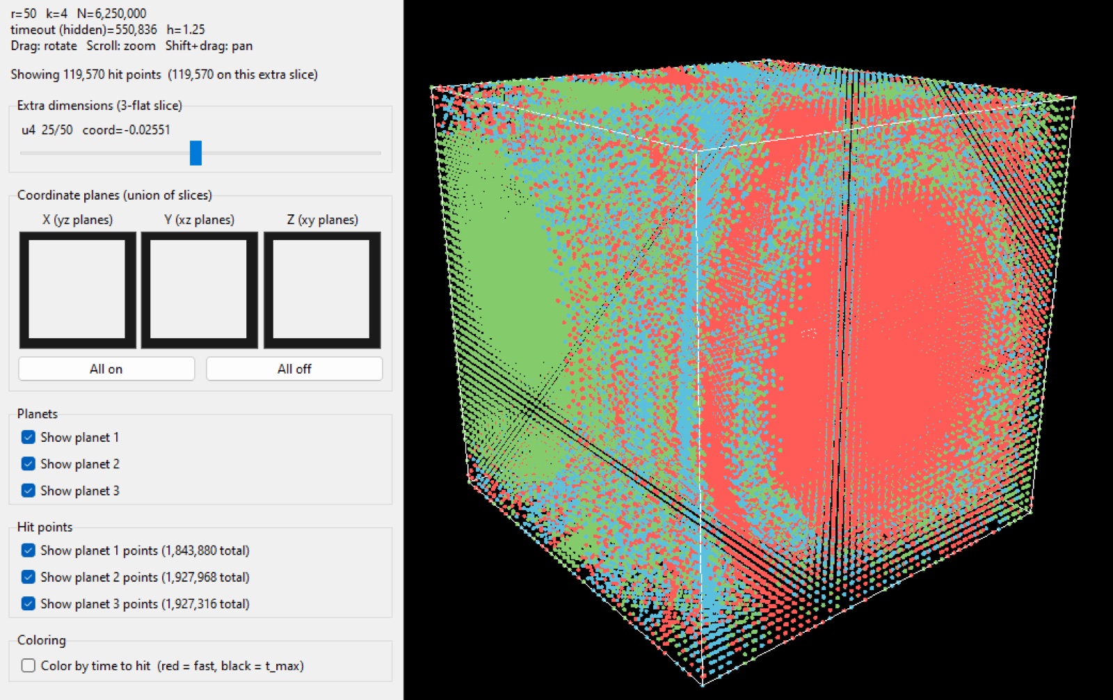
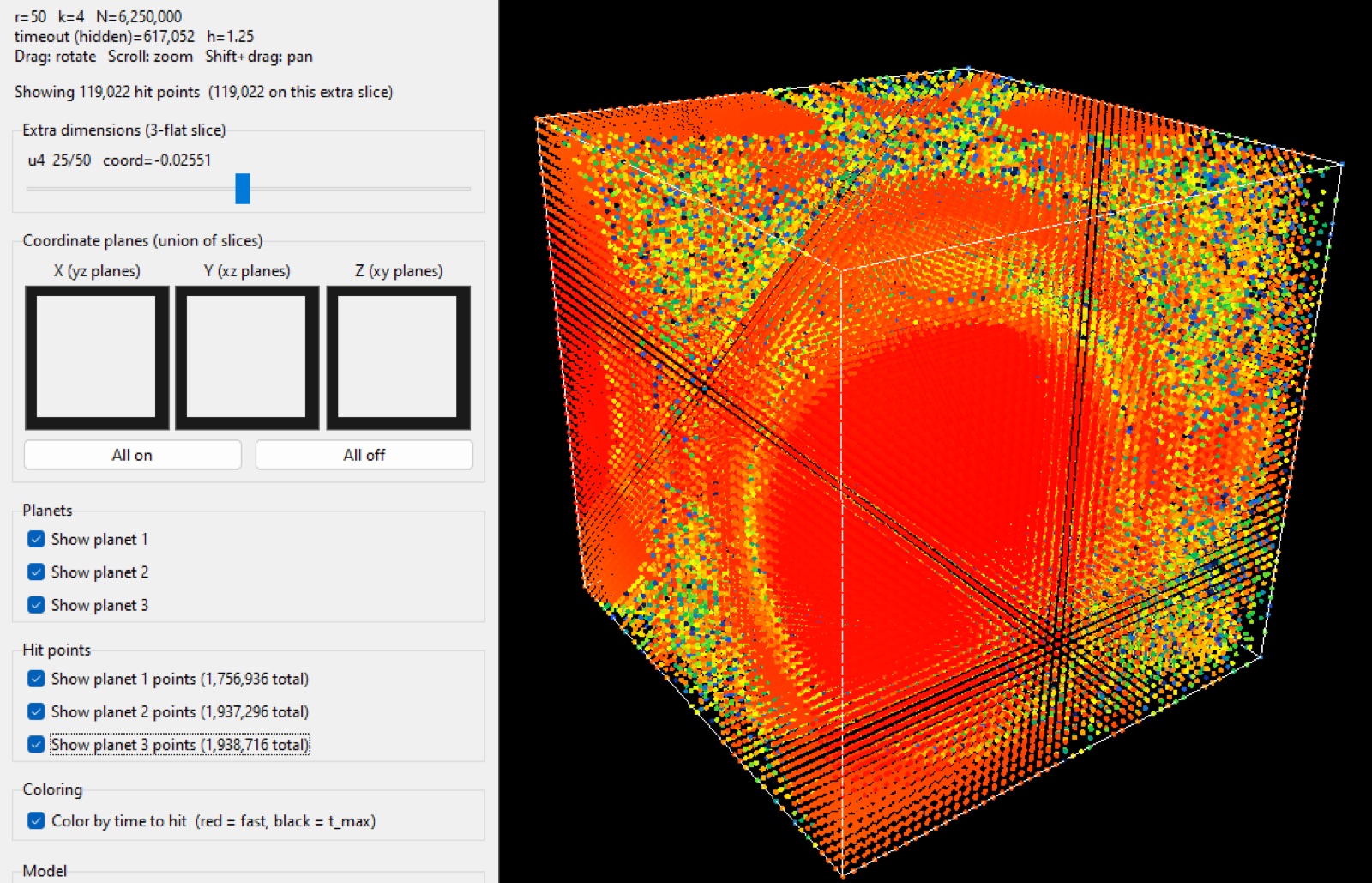
I never proved the Wada property to $\varepsilon\text{--}\delta$ . I just observed this pattern by zooming in on a boundary in which the basins appear to continuously keep appearing in between the boundaries. The images I obtained from this appear to follow Wada properties. The boundary is fractal in the practical sense that its apparent length grows under refinement and figuring out which planet an asteroid will hit if its initial position is on a boundary is unstable under arbitrarily small shifts of the initial point. Therefore there is a sensitive dependence. See Figures 1 and 4.

Colouring by time-to-hit makes the slow layer very obvious. The interiors of the lobes collide quickly (red). The filamentary sea takes much longer (green/blue). See Figure 3.

How I built the simulation

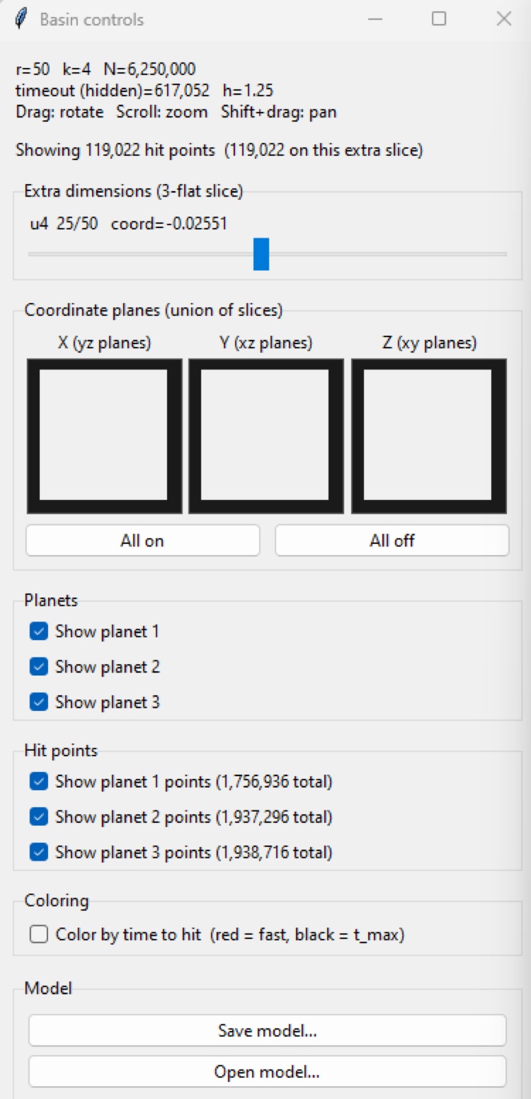
I used Python, NumPy, and CuPy. Each asteroid is an independent initial-value problem, so the natural parallelism is one asteroid per GPU block of work, compacting finished particles off the work set. Two-dimensional stills are rendered with Manim (pixel count is asteroid count). The n-D lattice is visualised with VisPy: a white 3-cube for the first three sampling axes, sliders are used for the rest, and a union of coordinate-plane slices. Each simulated run can be saved as an .npz file (initial lattice, hit index, collision time) and reopened without the need to re-simulate the system.

The VisPy Basin controls window: extra-dimension slider, coordinate-plane toggles, planet checkboxes and colouring options. — Figure 7. The viewer’s settings panel. Settings: VisPy “Basin controls” (extra-dimension slider, coordinate-plane unions, planet toggles, colour modes).

A first look at relativistic motion

See Figure 4. The relativistic flag was not the point of the programme, but it was the hardest piece of physics I had to get straight. What if the system was affected by relativistic motion? This was just another curious question I had and I wanted to see what it would change. I tried my best to implement this, I am not entirely sure if it is implemented properly but things look different, so it did something.

Exact multi-planet general relativity is not a closed-form metric. Einstein’s equations are nonlinear, so you cannot add Schwarzschild solutions for each mass and call the sum a spacetime. I wanted the asteroid to feel all of the frozen planets at once. The consistent choice, given planets held fixed by hand, is geodesic motion of a test particle in a prescribed static multi-mass field. The planets are boundary conditions, not a self-consistent 3-body geometry.

I took the Newtonian potential

\Phi(\mathbf{x}) = -\sum_i \frac{G m_i}{\lVert \mathbf{x} - \mathbf{p}_i \rVert},

put into the weak-field isotropic metric seen by a static observer at infinity,

g_{tt} \approx -\left(1 + \frac{2\Phi}{c^{2}}\right), \qquad g_{ij} \approx \left(1 - \frac{2\Phi}{c^{2}}\right)\delta_{ij},

and the 3-acceleration in coordinate time $t$ is then the standard 1PN geodesic form

\mathbf{a} = -\nabla\Phi\left(1 + \frac{v^{2}}{c^{2}} + \frac{4\Phi}{c^{2}}\right) + \frac{4\,\mathbf{v}\,(\mathbf{v}\cdot\nabla\Phi)}{c^{2}}.

Two consequences are immediate and were new to me in practice. First, $\mathbf{a}$ depends on velocity, so the integrator’s RK4 stages must evaluate $\mathbf{a}(\mathbf{x},\mathbf{v})$ at each stage. Acceleration as a function of position alone is the Newtonian special case. Second, the expansion is only a controlled correction to Newton when $|\Phi|/c^{2} \ll 1$ and $|v|/c \ll 1$ . In these units ( $G \sim 1$ , sizes $\sim 1$ ) Newtonian speeds are order one, so $c$ cannot be huge or the flag is invisible. If instead $2GM/c^{2}$ is comparable to a planet’s radius, the same formula is being used outside its derivation. That is what the “weak-field geodesic is a toy” warning means. The picture is still coloured in coordinate time: there is no lensing, no time-dilated photograph.

I learnt that you do not “turn on relativity” by adding extra $1/r^{2}$ terms at random, and you do not get a 3-body spacetime by superposing black holes. You pick a metric, write the geodesic equation in a definite time coordinate, and stay honest about the regime of the approximation. Implementing it meant accepting an approximate geodesic law and stating clearly where that approximation stops being a small correction.

The 4-D viewer with the geodesic flag on, showing a distinctly different ring-like structure inside the cube. — Figure 8. Geodesic flag on, visualised in 4-D. Notice the physical difference between Figure 5 and Figure 8. Settings: geodesic flag true, time-to-hit flag false, visualised in 4-D.

What the programme is made for

This is quite a poor model of orbital mechanics. The planets do not orbit each other, the asteroids start at rest, there is no radiation pressure, no oblateness, no third-body ephemeris, and the quantity of interest is the endpoint of a collision, not its trajectory. Thus it is very unrealistic in that sense.

I built this programme for the chaotic scattering of masses and the visualisation of the gravitational basin boundaries. A deterministic Newtonian system whose long-term fate, as a function of initial position, is fractal and (in the three-colour case) Wada-like. That is the same mathematical species as other open Hamiltonian exit problems.

It is also a data-visualisation problem. The object of interest is a function from a region of $\mathbb{R}^{n}$ to a discrete label (or to a time). For $n > 3$ you cannot see it at once since we live in 3-dimensional space. I decided to use 2-flats, 3-flats, extra-coordinate sliders so that you can effectively slide through the 4th dimension and see how the basin changes. There are also two different colourings of the same samples. Visualising $(n-1)$ -spheres by their intersection with the current flat is the same idea applied to the planets themselves.

What I learnt

Rotations in $n$ dimensions are $SO(n)$ , with $\tfrac{n(n-1)}{2}$ degrees of freedom. The most important part is that it is quadratic, not linear. Big misconception I believed.

I learnt that these systems aren’t as simple as Voronoi diagrams. They are fractals where the boundary appears to behave like a Wada boundary. The chaos here is not random either. It is deterministic motion whose endpoint, as a map from initial data, is unstable at every scale.

The 1PN geodesic made it clear that relativistic motion is motion in a metric. The Newtonian limit is a controlled expansion in $v/c$ and $\Phi/c^{2}$ , and that a spacetime with multiple masses is not as simple as the sum of one-body solutions. Implementing required me to use an approximate geodesic law and stating clearly where that approximation stops being a small correction.

On the engineering side I learnt that a visualisation of high-dimensional data is only as honest as the cross section you chose, and that it all pretty much depends on your frame of reference. You can't just choose a random cross section and expect the results to be meaningful.

The 4-D viewer coloured by time-to-hit: a warm red core wrapped in a slower yellow-green shell. — Figure 9. Coloured by time-to-hit, visualised in 4-D. Settings: geodesic flag false, time-to-hit flag true, visualised in 4-D.

The 4-D viewer showing only the points that collide with the red planet. — Figure 10. Only the set of starting points that collide with the red planet. Settings: geodesic flag false, time-to-hit flag false, visualised in 4-D, red-planet hits only.

References

These pages helped a lot with researching for this project. Also fun to read.

History Topics: Mathematical Physics Index — MacTutor History of Mathematics, University of St Andrews
Relativity: The Special and General Theory — Albert Einstein
Testing Chern-Simons modified gravity with orbiting superconductive gravity gradiometers — Li-E Qiang and Peng Xu, arXiv:1502.04632, 2015
Post-Newtonian N-body dynamics in Extended Theories of Gravity — Antonio Tedesco, The European Physical Journal C, 2026
Theory of Continuous Set of Points — Kunizô Yoneyama, Tohoku Mathematical Journal, 1917
On the creation of Wada basins in interval maps through fixed point tangent bifurcation — Romulus Breban and Helena E. Nusse, Physica D, 2005
Special orthogonal group — Wolfram MathWorld
Chaos — Wolfram MathWorld

Back home